Feature engineering is a crucial aspect of the machine learning process. It involves creating new features or transforming existing ones to enhance the performance of a model. In this tutorial, we will delve into the basics of feature engineering with Python and how to create relevant features.
Step 1: Understanding the Data
Before creating features, it is essential to comprehend the data we are working with. We need to understand the data type, its distribution, and any missing values. This information will guide us in determining the best approach to creating features.
To understand the data, we can use several techniques such as data visualization and statistical tests. Data visualization helps us identify patterns and relationships between variables. For instance, we can create scatter plots to visualize the connection between two continuous variables, or bar charts to visualize the distribution of a categorical variable. Statistical tests, such as correlation analysis, help us identify the strength and direction of the relationship between two variables.
Step 2: Feature Creation
Once we have a good understanding of the data, we can start creating features. There are several techniques we can use to create new features, including:
- One-Hot Encoding
- Binning
- Feature Scaling
1. One-Hot Encoding
One-hot encoding is a technique used to convert categorical variables into numerical features. It creates a new binary feature for each unique value in the categorical variable. For instance, if we have a categorical variable called “color” with values “red,” “green,” and “blue,” one-hot encoding would create three new binary features: “color_red,” “color_green,” and “color_blue.”
One-hot encoding is useful when we have categorical variables with no inherent order or hierarchy. It helps capture the unique information in each category and avoid assigning arbitrary numerical values to each category.
However, one-hot encoding can lead to the curse of dimensionality, which is when the number of features becomes too large compared to the number of observations. This can lead to overfitting and reduced performance of the model.
2. Binning
Binning is a technique used to group continuous variables into discrete intervals. It can help capture non-linear relationships between the feature and the target variable. For example, we can bin a variable called “age” into categories such as “child,” “teenager,” “adult,” and “senior.”
Binning is useful when we have continuous variables that exhibit non-linear relationships with the target variable. It helps simplify the relationship between the feature and the target variable and reduce the noise in the data.
However, binning can lead to loss of information and reduced granularity. It can also be sensitive to the choice of bin sizes and boundaries.
3. Feature Scaling
Feature scaling is a technique used to normalize the range of values in a feature. It can help improve the performance of models that are sensitive to the scale of the features. There are several methods for feature scaling, including standardization and min-max scaling.
Feature scaling is useful when we have features with different scales or units of measurement. It helps ensure that each feature contributes equally to the model and avoid bias towards features with larger scales.
However, feature scaling can lead to loss of information and reduced interpretability. It can also be sensitive to the presence of outliers in the data.

Step 3: Feature Selection
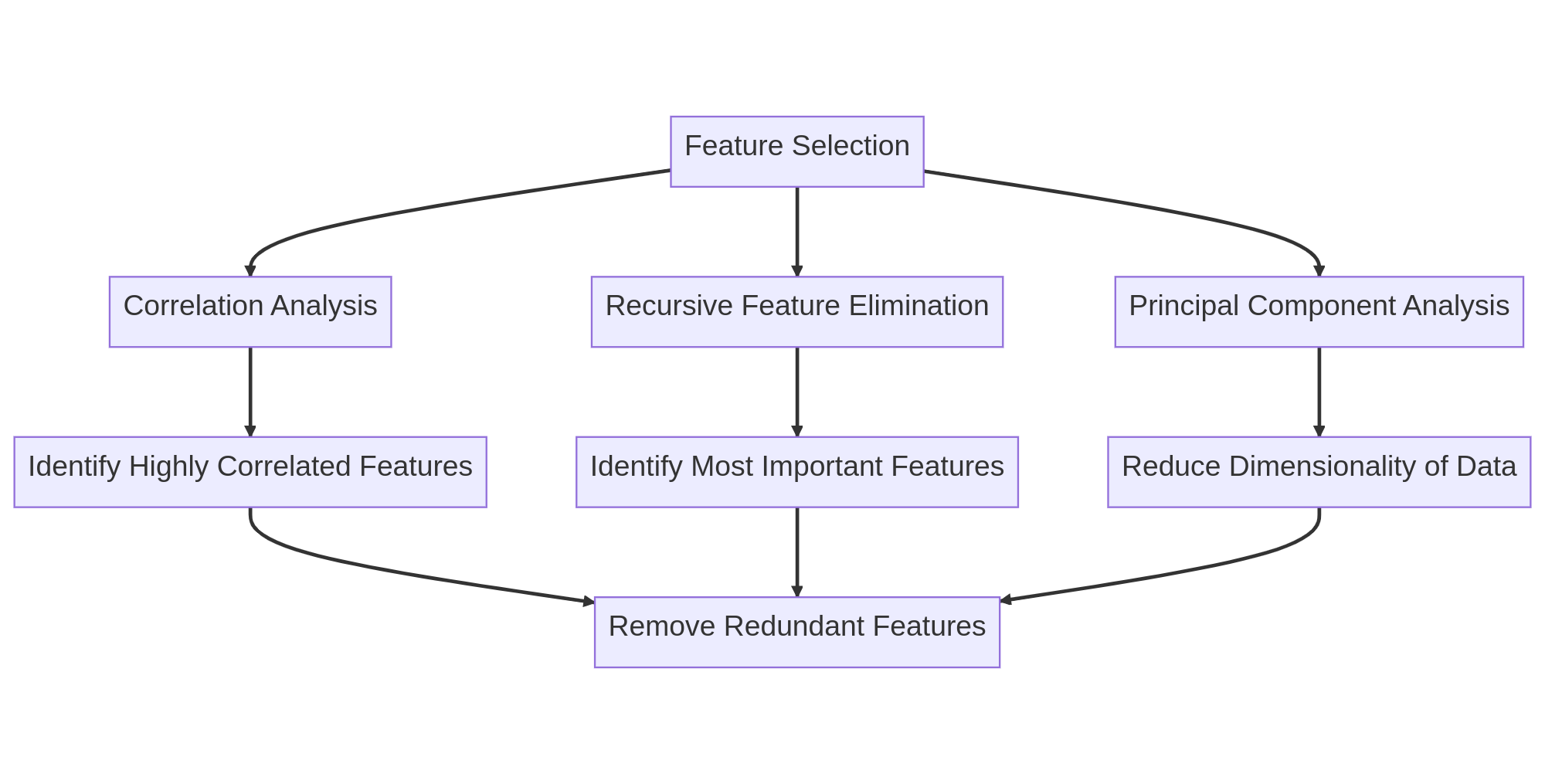
After creating new features, we need to select the ones that are most relevant to the target variable. Feature selection helps reduce the dimensionality of the data and improve the performance of the model. There are several techniques for feature selection, including:
- Correlation Analysis
- Recursive Feature Elimination
- Principal Component Analysis
1. Correlation Analysis
Correlation analysis measures the strength of the relationship between two variables. We can use it to identify features that are highly correlated with the target variable and remove features that are redundant.
If a feature is highly correlated with the target variable, it means that it contains valuable information for predicting the target variable. However, if two features are highly correlated with each other, it means that they contain redundant information and can be removed to reduce the dimensionality of the data.
2. Recursive Feature Elimination
Recursive feature elimination is a technique that recursively removes features and fits the model again until the optimal number of features is reached. It can help identify the most important features for the model.
Recursive feature elimination helps identify the features that have the most predictive power for the target variable. However, it can also be computationally expensive and may not be feasible for large datasets.
3. Principal Component Analysis
Principal component analysis is a technique used to reduce the dimensionality of the data by transforming the features into a new set of variables called principal components. It can help identify the features that explain the most variance in the data.
Principal component analysis helps identify the underlying patterns and structure in the data. However, it can also be difficult to interpret the meaning of the principal components and may not be suitable for datasets with highly correlated features.

Step 4: Implementing Feature Engineering in Python
Now that we have a good understanding of feature engineering, let’s implement it in Python. We will use the scikit-learn library, which provides several tools for feature engineering and selection.
As an example, we will use the Boston Housing dataset, which contains information about the housing values in suburbs of Boston. The dataset has 13 features, including the crime rate, average number of rooms per dwelling, and pupil-teacher ratio by town.
First, we will load the data and split it into training and testing sets:
from sklearn.datasets import load_boston
from sklearn.model_selection import train_test_split

data = load_boston()
X_train, X_test, y_train, y_test = train_test_split(data.data, data.target, test_size=0.2, random_state=42)
Next, we will create new features using one-hot encoding and binning:
from sklearn.preprocessing import OneHotEncoder, KBinsDiscretizer

# One-hot encoding
encoder = OneHotEncoder(sparse=False)
X_train_color = encoder.fit_transform(X_train[:, 3].reshape(-1, 1))
X_test_color = encoder.transform(X_test[:, 3].reshape(-1, 1))

# Binning
bins = KBinsDiscretizer(n_bins=4, encode='ordinal', strategy='quantile')
X_train_age = bins.fit_transform(X_train[:, 6].reshape(-1, 1))
X_test_age = bins.transform(X_test[:, 6].reshape(-1, 1))
Finally, we will select the most relevant features using correlation analysis and recursive feature elimination:
from sklearn.feature_selection import SelectKBest, f_regression, RFE
from sklearn.linear_model import LinearRegression

# Correlation analysis
selector = SelectKBest(score_func=f_regression, k=5)
X_train_corr = selector.fit_transform(X_train, y_train)
X_test_corr = selector.transform(X_test)

# Recursive feature elimination
estimator = LinearRegression()
selector = RFE(estimator, n_features_to_select=5)
X_train_rfe = selector.fit_transform(X_train, y_train)
X_test_rfe = selector.transform(X_test)
Conclusion
Feature engineering is a critical step in the machine learning process. It helps improve the performance of models and capture non-linear relationships between features and the target variable. In this tutorial, we explored the basics of feature engineering with Python and how to create relevant features. We also learned how to select the most relevant features using correlation analysis and recursive feature elimination. With these techniques, we can build more accurate and robust machine learning models.


